Python Exceptions: Part Three


exceptionsIn the previous articles, we covered the try and except clauses. In this article, we will start out by looking at the else clause.

Python Exceptions: The Else Clause

Although the purpose of the else clause may not be readily apparent, it is necessary because without it, there is no way to tell whether the flow of control has proceeded past a try statement because no exception was raised, or because an exception occurred and was handled – at least not without setting and checking Boolean flags. Much like the way else clauses in loops make the exit cause more apparent, the else clause provides syntax in a try that makes what has happened obvious and unambiguous. For example:

try:
# Run some code
except SomeError:
# Handle the exception
else
# No exception has occurred

You can do something similar by moving the else code into the try block. This can lead, however, to incorrect exception classifications. If the “no exception occurred” action triggers a SomeError, it will register as a failure of the try block and erroneously trigger the exception handler below the try. By using an explicit else clause instead, you will make the logic more obvious and guarantee that except handlers will run only for real failres in the code you are wrapping in a try, not for failures in the else case’s action.

The other variant of the try statement is a specialization that has to do with finalization actions. If a finally clause is included in a try, Python will always run its block of statements “on the way out” of the try statement, whether an exception occured while the try block was running or not. Its general form is:

try:

finally:

With this variant, Python begins by running the statement block associated with the try header line. What happens next depends on whether an exception occurs during the try block. If no exception occurs while the try block is running, Python jumps back to run the finally block and then continues execution past below the try statement. If on the other hand an exception does occur during the try block’s run, Python still comes back and runs the finally block, but it then propagates the exception up to a higher try or the top-level default handler; the program does not resume execution below the try statement. That is, the finally block is run even if an exception is raised, but unlike an except, the finally does not terminate the exception – it continues being raised after the finally block runs.

The try/finally form is useful when you want to be completely sure that an action will happen after some code runs, regardless of the exception behavior of the program. In practice, it allows you to specify cleanup actions that always must occur (such as file closes).

Note that the finally clase cannot be used in the same try statement as except and else in Python 2.4 and earlier, so the try/finally blocks are best thought of as a distinct statement form if you are using an older version of Python. In Python 2.5 and later, however, finally can appear in the same statement as except and else, so today there is essentially a single try statement with many optional clauses. Whichever version you use, though, the finally clause still serves the same purpose: to specify cleanup actions that must always be run, regardless of any exceptions.

External Links:

Handling Exceptions at Python Wiki

Built-in Exceptions at docs.python.org

Python Exceptions: Part Two

exceptionsIn the previous article, we covered some of the basics of exception handling in Python. In this article, we will go into a bit more detail on exception processing, and explore the details behind the try, raise, assert, and with statements.

Python Exceptions: Try, Raise, and Assert

We will start with the try statement, introduced in the previous article. The try statement is a compound statement which starts with a try header line, followed by a block of usually indented statements, then one or more except clauses that identify exceptions to be caught, and an optional else clause at the end. The words try, except and else are associated by indenting them to the same level. For example:

try
	statements
except name1:
	statements
except name2 as something:
	statements
except:
	statements
else:
	statements

Here, the block under the try header represents the main action of the statement. This is the code you are trying to run. The except clauses define handlers for exceptions raised during the try block. The else clause, if coded, provides a handler to be run if no exceptions occur.

When a try statement is entered, Python marks the current program context so it can return to it if an exception occurs. The statements nested under the try header are run first. What happens next is dependent on whether exceptions are raised while the try block’s statements are running. If an exception does occur while the try block’s statements are running, Python jumps back to the try and runs the statements under the first except clause that matches the raised exception. Control resumes below the entire try statement after the except block runs, unless the except block raises another exception. But if an exception happens in the try block and no except clause matches, the exception is propagated up to the last matching try statement that was entered in the program, or (if it’s the first such statement) to the top level of the process. If it is at the top level of the process, Python will stop the program and print a default error message. Finally, if no exception occurs while the statements under the try header run, Python runs the statements under the else line, if there are any, and control then resumes below the entire try statement.

except clauses catch exceptions that occur only within the statements in the associated try block. As such, they are considered focused exception handlers. However, since the try block’s statements can call functions coded elsewhere in a program, the source of an exception may be outside the try statement itself.

There are several clauses you can use after the try header, but you have to use at least one. In addition, you can code else only if there is at least one else. There can be several except clauses, but there can only be one else and one finally. Through Python 2.4, the finally clasue must appear alone, without an else or except. As of Python 2.5, however, a finally can appear in the same statement as except and else.

Because Python looks for a match within a given try by inspecting the except caluses from top to bottom, the parenthesized version has the same effect as listing each exception in its own except clause, but with the benefit of only having to code the statement body once.

The empty except clause is a sort of wildcard feature; it catches everything. Therefore, it allows your handlers to be as general or specific as you like. This may be more convenient than listing all possible exceptions in a try. But empty except clasues raise some design issues. Although they are convenient, they may catch unexpected system calls unrelated to your code. For example, even system exit calls in Python trigger exceptions, and you usually want them to pass. For that reason, Python 3.0 introduced an alternative. Catching an exception named Exception has almost the same effect as an empty except, but ignores exceptions related to system exits. Other system calls, however, may still trigger exceptions.

External Links:

Handling Exceptions at Python Wiki

Built-in Exceptions at docs.python.org

Python Exceptions: Part One

exceptionsExceptions are events that can modify the flow of control through a program; they are triggered automatically on errors, and can be triggered and intercepted by your Python code. Python has the following statements to deal with exceptions:

  • try/except: Catch and recover from exceptions raised by Python (or by you)
  • try/finally: Perform cleanup actions, whether exceptions occur or not.
  • raise: Trigger an exception manually in your code.
  • assert: Conditionally trigger an exception in your code.
  • with/as: Implement context managers in Python 2.6/3.0.

Exceptions let us jump out of large chunks of a program (whatever is included in the “try” block). The try statement works as follows:

  • First, the try clause is executed.
  • If no exception occurs, the except clause is skipped and execution of the try statement is finished.

To provide an example, let’s assume we have a character string:

>>> myStr = ‘Hello, world!’
>>> print(myStr[3])
l

If we reference an index within the bounds of the string, then the code works as it should, and we get no error. But if we specify an index outside of the bounds of the string, we get a different result:

Traceback (most recent call last):
File “<pyshell#3>”, line 1, in
print(myStr[13])
IndexError: string index out of range

Handling Exceptions

In our programs, we can let an error occur, in which case the program stops running, or we can try to handle it. The error generated by trying to access myStr[13] was an IndexError, so we will handle the IndexError exception in our code:

def testException():
	myStr = 'Hello, world!'
	try:
		print(myStr[13])
		print('No errors so far.')
	except IndexError:
		print('Index error.')
	print('Continuing...')

In this code, we have a try/except block. In try, we attempt to print out myStr[13]. If there is no error, we will move on to the next line (and print out ‘No errors no far.’). If an IndexError exception is raised, we will jump immediately to the except statement. The last line (print out ‘Continuing…’) will execute whether or not an exception was raised. Not surprisingly, we get the following output when we run the function:

>>> testException()
Index error.
Continuing…

Note that if the program generated an exception that was not an IndexError, the exception would be unhandled and the program would terminate with an error. However, a try statement may have more than one except clause, to specify handlers for different exceptions. At most one handler will be executed. Handlers only handle exceptions that occur in the corresponding try clause, not in other handlers of the same try statement. An except clause may also name multiple exceptions as a parenthesized tuple. For example:

except (IndexError, ValueError, RuntimeError):
pass

In this case, the last except clause may omit the exception name or names to serve as a wildcard. You can use this to print an error message and re-raise the exception to allow the caller to handle the exception as well. For example, we could rewrite the above function:

def testException():
    myStr = 'Hello, world!'
    try:
        print(myStr[12])
        print('No errors so far.')
        a = int(myStr[12])
    except IndexError:
        print('Index error.')
    except ValueError:
        print('Value error.')
    print('Continuing...')

If we execute this function, we get the following result:

>>> testException()
!
No errors so far.
Value error.
Continuing…

The first print() call in the try block will not raise an exception, but trying to convert myStr[12] to an integer will generate a ValueError exception.

You can also add a finally block to your code. The finally block is inserted after the try block and is executed whether or not an exception is generated (and whether or not said exception is handled). For example, we might have the following function:

def testException():
    myStr = 'Hello, world!'
    try:
        print(myStr[12])
        print('No errors so far.')
        b.append(myStr[12])
    except IndexError:
        print('Index error.')
    except ValueError:
        print('Value error.')
    finally:
        print('Finally block reached.')
    print('Continuing...')

Here, the line with the b.append() call will generate an unhandled exception because b was not previously defined as a list. Thus, it will not reach the last line of the program, but it will execute what is in the finally block:

!
No errors so far.
Finally block reached.
Traceback (most recent call last):
File “N:\Users\David\workspace\exception\exception.py”, line 16, in
testException()
File “N:\Users\David\workspace\exception\exception.py”, line 7, in testException
b.append(myStr[12])
NameError: global name ‘b’ is not defined

Exception handling in Python is not unlike try/catch blocks in C++ and try/catch/finally blocks in Java. It provides a useful alternative to the old C approach, which was to propagate error codes:

int functionCall()
{
	if (doSomething() == ERROR_CODE)
		return ERROR_CODE;
}

void main()
{
	if (functionCall() == ERROR_CODE)
		badResult();
	else
		goodResult();
}

In this case, a lot of our code is devoted to error handling. If we had a try/except block, however, we could just wrap the code we think might cause an error in a try block.

We are not quite done examining exception handling in Python, but hopefully this will serve as a good introduction.

External Links:

Handling Exceptions at Python Wiki

Built-in Exceptions at docs.python.org

matplotlib: Part Two

matplotlib

In the previous article, I introduced matplotlib and some basic pylab statements that can be used to produce graphs. In this article, we’ll use matplotlib and some basic computation to understand experimental data.

numpy Arrays

One of the examples used previously was using pylab to plot a graph of compound interest. matplotlib would be fairly useless, however if it was only used to graph data for such functions, and especially if the plot function only accepted list input. One alternate way of providing input to the plot method is to use numpy.arange():

import random, pylab
import numpy

t = numpy.arange(0,10,.25)
pylab.plot(t,t,'bo')
pylab.show()

In this code fragment, we use numpy.arange, and provide as input three arguments: the minimum, the maximum, and the interval. We supply to plot() three arguments: t, t (again), and ‘bo’ for blue circles. The result is a linear graph where y = x, and the circles appear at intervals of .25.

You can perform some mathematical operations on numpy arrays. For example:

pylab.plot(t,t*2,’bo’)

multiplies the array by a factor of 2, so we get a graph where y = 2*x. We could also square or cube a numpy array, like so:

pylab.plot(t,t*2,’bo’)
pylab.plot(t,t*3,’bo’)

Since having two functions represented by blue dots might be confusing, you probably want to use something else:

pylab.plot(t,t*3,’bs’)

The plot() method can also accept as input the return value of a function. For example, assume that we have a function to return the cosine of a number:

def func(t):
return numpy.cos(2*numpy.pi*t)

Then we can plot the function with pylab:

pylab.figure(1)
pylab.subplot(211)
pylab.plot(t,func(t),’bo’)
pylab.show()

Invoking pylab.figure() is optional because figure(1) will be created by default. The pylab.subplot() method specifies numrows, numcols, and fignum where fignum ranges from 1 to numrows*numcols. The comma in the subplot command are optional if numrows*numcols < 10. Thus, subplot(211) is identical to subplot(2,1,1). If you want to place axes manually (not on a rectangular grid, use the pylab.axes() method, which allows you to specicy a location as axes([left, bottom, with, height]) where all values are in fractional (0 to 1) coordinates.

Another useful method is pylab.savefig, which allows us to save the graph. For example:

pylab.savefig(“cos.png”,dpi=200)

allows us to save the graph as cos.png, with a resolution of 200 dots per inch (dpi). You can also save the graph by clicking on the disk icon on the menu at the top of the graph when the graph displays. Allowed formats include PNG, JPEG, TIFF, SVG and PDF.

External Links:

matplotlib at Wikipedia

The official matplotlib site

Pyplot tutorial at matplotlib.org

Python (x,y) download site

matplotlib: Part One

matplotlib

matplotlib is a plotting library for the Python programming language and its numerical mathematics extension NumPy. It provides an object-oritented API for embedding plots into applications using general-purpose GUI toolkits.

Since it is designed to resemble MATLAB, the pylab interface makes matplotlib easy to learn for experienced MATLAB users. Some of the advantages of matplotlib over MATLAB include the following:

  • It is based on Python, a full-featured modern object-oriented programming language suitable for large-scale software development.
  • Free, open source (therefore, there are no license servers)
  • Native SVG support

Unfortunately, matplotlib was designed to work with Python, so it is hard or impossible to use in other languages. Also it heavily relies on packages such as NumPy and SciPy, so there are a number of dependencies.

Installing matplotlib

matplotlib is easy to install in Linux from the repositories. In Debian, Ubuntu, Mint and many other distributions, you just need to type:

sudo apt-get install python-matplotlib

In Fedora, Redhat and CentOS, it’s:

sudo yum install python-matplotlib

Under Windows, in addition to the standard Python installation, you will also need to install compatible versions of setuptools, NumPy, python-dateutil, pytz, pyparsing and six in addition to matplotlib. NumPy depends on files installed with Microsoft Visual C++ 2008 (for Python 2.6 to 3.2) or Microsoft Visual C++ 2010 (for Python 3.3 and 3.4), so you will need to have Visual C++ installed. If not, it may be easier to install one of the scipy-stack compatible Python distributions such as Python(x,y), Enthought Canopy, or Continuum Anaconda, which have matplotlib and many of its dependencies, plus other useful packages, preinstalled.

Installation of Python(x,y) is easy. Download the current version from the official pythonxy download site and run the installer (the installation notes also recommend that you uninstall any other Python distribution before installing it). The installer will present you with a few basic options, after which installation will proceed. Once installation is complete, you can utilize Python(x,y). This package includes a Python interpreter called iPython (you can access it by typing “ipython” at the command line). I chose to use Eclipse instead. Eclipse automatically detected the installation of Python(x,y), and asked if I wanted to use it as the default Python interpreter. I selected this option and proceeded.

We need some code to test matplotlab, so I wrote the following:

'''A short bit of code to test matplotlib
and display a graph'''
import random, pylab

def mpltest():
    dicerolls = []
    for i in range(10):
        x = int(random.random()*6+1)
        y = int(random.random()*6+1)
        dicerolls.append(x+y)
    pylab.plot(dicerolls,'ro')
    pylab.title('Result of dice rolls')
    pylab.xlabel('Trial #')
    pylab.ylabel('Outcome')
    pylab.show()

mpltest()

In mpltest, the first few lines just create a list called dicerolls and use iteration to add data for the dice rolls to the list. The next few lines introduce pylab and some of its functions. pylab.plot will cause the data to be plotted. The second parameter, ‘ro’, will cause only red circles to be shown (“red only”); since each dice roll is independent of the others, we don’t want a line to be drawn connecting the points. pylab.title allows the graph to have a title, and pylab.xlabel and pylab.ylabel creates labels for the x and y-axis, respectively. Nothing actually appears on the screen, though, until we call pylab.show, which we do on the last line of the function call.

It would be nice to graph a continuous function as well, so let’s graph the growth of $10,000 if we have 7 percent interest, compounded yearly:

def interest():
    principal = 10000.0
    interestRate = 0.07
    years = 10
    iValues = []
    for i in range(years+1):
        principal += principal*interestRate
        iValues.append(principal)
    pylab.plot(iValues)
    pylab.title('7% Growth, Compounded Annually')
    pylab.xlabel('Years of Compounding')
    pylab.ylabel('Value of Principal ($)')
    pylab.show()
    
interest()

The format of the function is similar to the first one, although we have replaced the dice rolls with the growth of principal over time. In pylab.plot, we want to have a line connecting the points, so the second parameter is omitted.

We can see the results in the screen capture on the side of this article. matplotlib does seem to work as advertised. We will post more articles about matplotlib in the future, but hopefully this will serve as a useful introduction.

External Links:

matplotlib at Wikipedia

The official matplotlib site

Pyplot tutorial at matplotlib.org

Python (x,y) download site

Python Sets: Part Two

Python setsIn part one of this series, we took a first look at sets, a relatively new core data type in Python. In this article, we will continue cover set methods, as well as a new literal format for sets.

In addition to expressions, the set object provides methods that correspond to the set operations. For example, the set add method inserts one item; update provides an in-place union, and remove deletes an item by value. Run a dir call on any set instance or the set type name to see all the available methods. Assuming we have mySet and otherSet from the previous article:

>>> mySet = set(‘hello’)
>>> otherSet = set([‘a’,’b’,’c’,’d’,’e’])

then we can perform these operations:

>>> si = mySet.intersection(otherSet)
>>> si
{‘e’}
si.add(‘MORE’)
si
{‘MORE’, ‘e’}
>>> si.update(set([‘X’,’Y’]))
>>> si
{‘X’, ‘MORE’, ‘e’, ‘Y’}
>>> si.remove(‘e’)
si
{‘X’, ‘MORE’, ‘Y’ }

As iterable containers, sets can also be used in operations such as len, for loops, and list comprehensions. Because they are unordered, however, they do not support sequence operations like indexing and slicing.

>>> for item in set('aeiou'):
        print(item * 4)

uuuu
iiii
oooo
aaaa
eeee

Although these set expressions generally require two sets, they often work with any iterable types, such as lists, tuples, and ranges. For example:

mySet.union([‘a’,’b’,’c’])
{‘b’, ‘l’, ‘c’, ‘o’, ‘a’, ‘e’, ‘h’}
mySet.intersection((‘e’,’l’,’p’))
{‘e’, ‘l’}

Using Curly Braces

Python 3.0 adds a new set literal form, using the curly braces formerly reserved for dictionaries. In 3.0 and above, the following are equivalent:

set([‘a’,’b’,’c’])
{‘a’, ‘b’, ‘c’}

Because sets are unordered, unique, and immutable, a set’s items behave much like a dictionary’s keys, and therefore the new syntax makes sense. Regardless of how a set is made, 3.0 and above displays sets using the new literal format. The set built-in is still required in 3.0 to create empty sets and to build sets from existing iterable objects, but the new literal format is convenient for initializing sets of known structure:

>>> {‘a’,’b’,’c’}
{‘c’, ‘b’, ‘a’}

>>> S = {‘a’,’e’,’i’,’o’,’u’}
>>> S.add(‘MORE’)
>>> S
{‘MORE’, ‘i’, ‘o’, ‘a’, ‘e’, ‘u’}

All the set processing operations discussed in the previous article work the same in 3.0 and above, but the result sets print differently:

>>> S1 = {‘a’,’b’,’c’}
>>> S1 & {‘a’,’c’}
{‘c’,’a’}
>>> {‘a’,’e’,’i’,’o’,’u’} | S1
{‘b’, ‘i’, ‘o’, ‘c’, ‘a’, ‘e’, ‘u’}
>>> S1 – {‘a’,’b’}
{‘c’}
>>> S1 > {‘a’,’c’}
True

Note that {} is still a dictionary in Python. Empty sets must be created with the set built-in, and print the same way:

>>> S1 – {‘a’,’b’,’c’}
set()
>>> type({})
<class ‘dict’>

>>> mySet = set()
>>> mySet.add(‘a’)
>>> mySet
{‘a’}

As in Python 2.6, sets created with 3.0 literals support the same methods, some of which allow general iterable operands that expressions do not:

>>> {‘a’,’b’,’c’} | {‘c’,’d’}
{‘c’, ‘b’, ‘a’, ‘d’}
>>> {‘a’,’b’,’c’} | [‘c’,’d’]
Traceback (most recent call last):
File “<pyshell#34>”, line 1, in
{‘a’,’b’,’c’} | [‘c’,’d’]
TypeError: unsupported operand type(s) for |: ‘set’ and ‘list’

>>> {‘a’,’b’,’c’}.union([‘c’,’d’])
{‘c’, ‘b’, ‘a’, ‘d’}
>>> {‘a’,’b’,’c’}.union([‘c’,’d’])
{‘c’, ‘b’, ‘a’, ‘d’}
>>> {‘a’,’b’,’c’}.union(set([‘c’,’d’]))
{‘c’, ‘b’, ‘a’, ‘d’}
>>> {‘a’,’b’,’c’}.intersection((‘c’,’e’,’f’))
{‘c’}
>>> {2,3,4}.issubset(range(-5,5))
True
>>>

External Links:

Set, frozenset at docs.python.org – Official documentation on sets and frozensets for Python 3.4

Python Sets: Part One

Python sets

No, not that kind of set.

One of the core Python data types that we did not mention in earlier articles that perhaps deserves some attention is the set. Sets are a recent addition to Python; they are neither mappings (dictionaries) nor sequences (strings, lists and typles). Sets are created by calling the built-in set function or using new set literals and expressions in 3.0, and they support the usual mathematical set operations.

Introduction to Sets

Creating a set can be done two different ways:

>>> mySet = set(‘hello’)
>>> otherSet = {‘a’,’b’,’c’,’d’,’e’}

len returns the number of unique set items, so we get:
>>> len(otherSet)
5
But if we run the same operation on mySet, we get:
>>> len(mySet)
4

>>> ‘h’ in mySet
True
>>> ‘i’ in mySet
False
>>> mySet.isdisjoint(otherSet)
False
>>> newSet = set(‘he’)
newSet.issubset(mySet)
True

Mathematical set operations are generally valid on sets:

>>> mySet, otherSet
({‘o’, ‘e’, ‘l’, ‘h’}, {‘e’, ‘d’, ‘b’, ‘a’, ‘c’})

>>> mySet & otherSet
{‘e’}

>>> mySet | otherSet
{‘e’, ‘h’, ‘o’, ‘d’, ‘b’, ‘c’, ‘a’, ‘l’}
>>> mySet – otherSet
{‘o’, ‘l’, ‘h’}

There are a few other operations. <= tests whether ever element in the left operand set is in the right operand set. For example: >>> newSet <= mySet
True

But what if we want to return False if the sets are equal? Then we use <:
>> newSet < mySet

True

>>> exactcopy = set(mySet)
>>> exactcopy < mySet

False

>>> exactcopy <= mySet

True

We can flip the operand around, and check to see if the left operand set is a superset of the right operand set:

>>> mySet > newSet
True
>>> mySet >= newSet
True

Sets are mutable; you can add and remove items with the add and remove methods:

>>> otherSet.add(‘f’)
{‘e’, ‘f’, ‘d’, ‘b’, ‘c’, ‘a’}
>>> otherSet.remove(‘c’)
>>> otherSet
{‘e’, ‘f’, ‘d’, ‘b’, ‘a’}

You can also iterate over a set. For example:
>>> for s in mySet:
print(s)

o
e
l
h

Since sets are mutable, there are some things we cannot do with them: for example, we cannot use them as dictionary keys. But objects of type frozenset are immutable. Therefore:

>>> unchangeableSet = frozenset(‘abc’)

Although we can’t add and remove items, we can perform the usual set operations on frozensets, or a combination of sets and frozensets:

>>> mySet | unchangeableSet
{‘o’, ‘e’, ‘b’, ‘h’, ‘c’, ‘a’, ‘l’}

For an example of using frozenset to create keys for a dictionary, here’s a sample:

>>> keySet = frozenset(‘abc’)
>>> names = [ ‘Able’, ‘Baker’, ‘Charlie’ ]
>>> myDict = { }
>>> i = 0
>>> for s in keySet:
myDict[s] = names[i]
i += 1

>>> print(myDict)
{‘a’: ‘Able’, ‘b’: ‘Baker’, ‘c’: ‘Charlie’}

Here, we created an immutable set called keySet, and a list of items to put in our dictionary. We iterate through the set, mapping items in the list to keys in keySet. When we print out the results, we see that each item was successfully mapped to a key.

In the next article, we will continue our look at sets.

External Links:

Set, frozenset at docs.python.org – Official documentation on sets and frozensets for Python 3.4

Python Debugging: An Overview

debugging

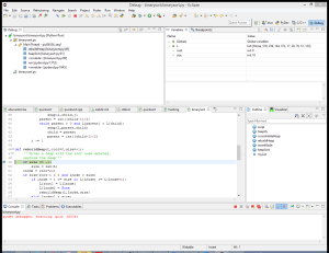
The Eclipse debugger in action.

At some point, one of your programs is likely to do something you did not expect it to do, and in such a scenario, you are going to have to debug your code. Fortunately, whether you are using the command line Python interpreter, the IDLE interface, or a third-party IDE, there are multiple options for debugging.

Debugging Options

One option is to rely on the error messages Python provides. If you already know Python, and especially if you understand your own code, this is often enough: you just read the error message and go and fix the tagged line and file. It may not always be a good option, however, for larger programs you did not write.

Another possibility, and probably the main way that Python programmers use for debugging their code is to insert print statements and run the program again. Because Python runs immediately after changes, this is usually the quickest way to get more information than error messages provide. Typically, a display of variable values is enough to provide the information you need.

For larger systems you did not write, and for beginners who want to trace code in more detail, most Python development GUIs have some sort of point-and-click debugging support. IDLE has a debugger as well, but it does not appear to be used very often (possibly because it has no command line, or possibly because adding print statements is usually quicker than setting up an IDLE GUI debugging session. But other IDEs such an Eclipse, NetBeans, Komodo and Wing IDE offer advanced point-and-click debuggers.

Python comes with a source-code debugger named pdb, available as a module in Python’s standard library. In pdb, you type commands to step line by line, display variables, set and clear breakpoints, or continue to a breakpoint or error. It can be launched interactively by importing it, or as a top-level script. Either way, it provides a powerful debugging tool.

To provide a real-world example of debugging to solve a coding problem, I introduced a bug into the binary sort code. The code is provided here; some readers may be able to find the bug just by looking at the code. In any case, when we run the code, we get the following result:

[None, None, 17, 144, 372, 51, 79, 123, 519, 997]

This result is wrong for at least two reasons. First, two list members have been replaced with “None”. Secondly, the list is not sorted. Fortunately, this gives us an opportunity to use our debugging skills. The heapSort function does the following:

  1. Creates a binary heap.
  2. While there is at least one item on the heap, delete the top item from the heap. If there is remaining heap data, rebuild the heap, consolidate the heap, and repeat this step.

A cursory review of the code seems to indicate that we correctly deleted the top item and re-inserted it after the heap. The error must be in heapify, rebuildHeap, or consolidateHeap. For starters, I decided to set a breakpoint after heapify is called and check to see if it returns a valid binary heap. If it does, we can be pretty sure the error is in rebuildHeap or consolidateHeap.

In Eclipse, I set a breakpoint in the second line of heapSort by right mouse-clicking on the left column next to that line of code (the column containing numbers indicating what line of code it is) and selecting “Add Breakpoint). Now I was able to debug the code by pressing “F11”. Eclipse now presents a dialog box asking if I want to switch to the debug perspective. Since I do, I press “Yes” and continue.

In the upper right corner of the Debug perspective, there is a section with two tabs: “Variables” and “Breakpoints”. The “Variables” tab provides us the information about local variables, including the current values stored in L. We can confirm that the list items form a valid binary heap:

        997
      /     \
    519     239
   /  \     / \
  144  372 17 29
  / \   /
79  51 123

It does not appear that the problem is in heapify, so it must be in either rebuildHeap or consolidateHeap. To find the bug, we will first step through the heapSort function line by line, by pressing F6.

As soon as we press F6 the first time, the variable high shows up on the variable list, since it has now made its first appearance in the code. The same goes for temp, when it makes its first appearance two lines later. The next line deletes the top node, and the change is reflected in the values for L shown on the “Variables” tab. All is well so far.

But after we run rebuildHeap for the first time, it is a different story. Our “heap” looks like this:

          519
         /   \
      None    29
      /  \    / \
    144  372 17 None
    / \   /
   79 51 123

It looks like rebuildHeap has failed us. Nodes marked “None” should not have children. The next step will be to remove the breakpoint from heapSort and put a breakpoint in rebuildHeap. Then we will restart the program. We terminate the program by pressing “CTRL-F2” and then pressing “F11” again.

Once we do this, we can continue debugging and begin stepping through the source code again. Looking at the “Variables” tab, we can see that lnode (left node) is initially set to 1, the correct value for the left node of the root node. The next line checks to see if there is at least one heap item and a left node. There is, so we proceed to the next line. We have to promote either the left node or the right node. We promote the left node if it is greater than the right node or if there is no right node. If so, we assign the left node’s value to the root node, mark the left node as empty, and run rebuildHeap recursively on the left node. When we reach the recursive rebuildHeap call, we will use “F5” to step into the second copy of rebuildHeap.

Once we start stepping into the second rebuildHeap, we can see something is wrong. lnode is now 5, but as the lnode of the lnode of the root, it should be 3. This is because root is equal to 2 when it should be 1. Looking at the first recursive rebuildHeap call in the function, we see that the second parameter is lnode+1 (which calls the function recursively on the right node), when it should be lnode (to call the function recursively on the left node). If we keep stepping through the code, rebuildHeap will perform operations on the wrong nodes and tamper with the integrity of heap data that should be kept intact. Here, it will promote one of the children of the right node, and erase data, as we can see by viewing list L’s values just before the next rebuildHeap call:

[519, None, 29, 144, 372, 17, None, 79, 51, 123]

In other words, it looks this is what accounts for the error in rebuildHeap. We could continue to step through the code, but to save time, let’s change the second rebuildHeap parameter at line 56 to lnode, remove the breakpoint, and see what happens.

Running the program after that modification results in the following output:

[17, 29, 51, 79, 123, 144, 239, 372, 519, 997]

Thus, it seems as if we have isolated and fixed the bug that was causing the error we were seeing earlier. This does not guarantee that our code is bug-free, but if there are other bugs to be found, we can have some confidence that the methods used here can be applied to finding them.

In this example, we used the Eclipse debugger for debugging, but don’t let this discourage you from using whatever tools you want. The Winpdb system, for example, is an open source stand-alone debugger with advanced debugging support and cross-platform GUI and console interfaces. These options become more important as you start writing larger scripts, but at least Python’s debugging support makes the process of finding errors a lot easier than they might be otherwise.

External Links:

The official Eclipse web site – An excellent IDE with good debugging capabilities

The official Winpdb web site

Classes and Inheritance: Part Two

classesIn the previous article, we introduced Python classes, discussed some of their features, and some of the similarities and differences from C++ classes. In this article, we will use our knowledge of C++ classes to rewrite our hash functions as a Python class.

Writing the HashObject Class

Our first job is to write the class constructor. Since it makes sense to initialize our list when the class is first instantiated, I decided to incorporate the createBuckets() function as part of the constructor:

class HashObject(object):
    def __init__(self, num):
        self.numBuckets = num
        self.hashSet = []
        for i in range(num):
            self.hashSet.append([])

This constructor takes one parameter (num), and assigns it to numBuckets, and then initializes our list.

Next, we want to define hashElement, which takes a number and hashes it to an index in hashSet. This function is the same as before, except that we do not have to pass the number of buckets to it:

def hashElement(self, elem):
        if type(elem) == int:
            return elem%self.numBuckets

The new insert function requires only one parameter: the list item to be inserted into one of the buckets:

def insert(self, i):
        self.hashSet[self.hashElement(i[0])].append(i)

Note that it is assumed that the first element of the list to be stored is assumed to be the key. Next, we need a remove function. We will take one parameter: the key value of the item to be deleted:

def remove(self, key):
        newElement = []
        for j in self.hashSet[self.hashElement(key)]:
            if j[0] != key:
                newElement.append(j)
        self.hashSet[self.hashElement(key)] = newElement    

Finally, we need to write the function to check to see if an item with a certain key exists:

def member(self, key):
        return i in self.hashSet[hashElement(key)]

One additional member function we may want to define is an accessor function for hashSet so we do not have to directly access the list, a good practice, since data hiding is one of the objectives of object-oriented programming:

def getElement(self, key):
        for j in self.hashSet[self.hashElement(key)]:
            if j[0] == key:
                return j

As you can see, we iterate through each list item in the bucket the key value hashes to (multiple items may be stored in a single bucket). When we find an item whose first value equals the key, we return that item.

With variables and member functions for HashObject defined, we can rewrite hashTest to test our class:

def hashTest():
    h = HashObject(51)
    h.insert([2175,'Homer Simpson','Technician',20])
    print(h.getElement(2175))
    h.insert([4158,'Elmer Higgins','Engineer',17])
    print(h.getElement(4158))
    h.insert([2583,'Waylon Smithers','Assistant',25])
    print(h.getElement(2583))
    h.remove(2175)
    print(h.getElement(2175))
    print(h.getElement(2583))

Running this function results in the following output:

[2175, ‘Homer Simpson’, ‘Technician’, 20]
[4158, ‘Elmer Higgins’, ‘Engineer’, 17]
[2583, ‘Waylon Smithers’, ‘Assistant’, 25]
None
[2583, ‘Waylon Smithers’, ‘Assistant’, 25]

In this function, we first create a hash set with 51 buckets. We insert the first record (Homer Simpson’s), and print it out, confirming its successful insertion. We insert a second record, also printing it out to confirm its insertion. Then we enter a third item (which, incidentally, hashes to the same location as the first item), and print it out, confirming its insertion and also confirming that we can successfully iterate through a bucket. Finally, we remove the first record and try to print it out. Since the getElement function will not return a value for a nonexistent record, the print call prints out “None”, for no value. Finally, we successfully print out the third record.

I have made HashObject and HashTest available for download here, so you can download it, run it and modify it to your heart’s content.

External Links:

Classes Tutorial on python.org

Class (computer programming) on Wikipedia